HIGHWAY QUALITY TEST

Precision Testing. Proven Quality. Safer Infrastructure.

Kinematic Viscosity Test of Bitumen – Step-by-Step Procedure, Formula, Calculation & Precautions

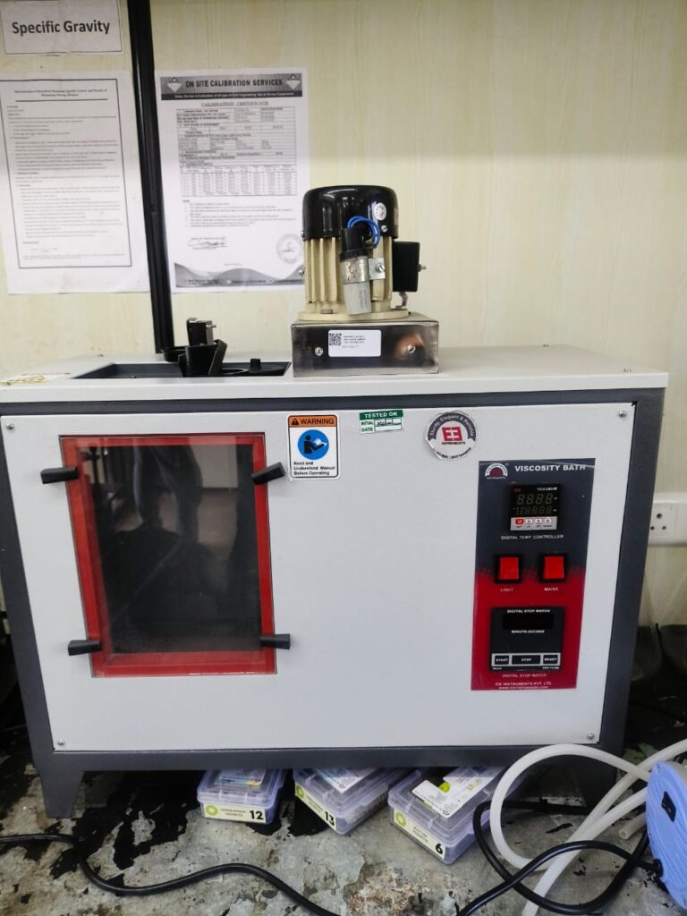
Determination of Kinematic Viscosity of Bitumen The Kinematic Viscosity Test is conducted to determine the resistance of bitumen to flow under the influence of gravity at a specified temperature. The test is performed using a Glass Capillary Viscometer and is widely used for quality control of paving bitumen in highway construction projects. In major highway projects executed by leading EPC contractors, including L&T ECC Division, the test is carried out during material approval, source verification, quality assurance, and routine laboratory testing to ensure that the bitumen possesses the required flow characteristics for mixing, pumping, spraying, and compaction. Objective To determine the kinematic viscosity of bitumen for: Material Approval Quality Control Testing Bitumen Source Verification Highway Pavement Construction Batch Acceptance Testing Compliance with IS and IRC Specifications Apparatus Required Glass Capillary Viscometer (Cannon-Fenske or equivalent) Constant Temperature Bath Thermometer Vacuum or Suction Device Stopwatch (0.1 second accuracy) Heating Oven Beaker Cleaning Solvent Drying Oven Principle The test is based on measuring the time required for a fixed volume of bitumen to flow through a calibrated glass capillary viscometer under gravity at a specified constant temperature. The flow time is multiplied by the viscometer constant to obtain the Kinematic Viscosity, expressed in mm²/s (centistokes, cSt). Detailed Testing Procedure The following procedure is commonly adopted in highway material laboratories for determining the Kinematic Viscosity of Bitumen using a calibrated glass capillary viscometer in accordance with ASTM D2170 / IS requirements. Step 1 – Selection of Viscometer Select a clean, calibrated Glass Capillary Viscometer (Cannon-Fenske, BS U-Tube or equivalent) having a suitable viscometer constant for the expected viscosity range. Verify that the viscometer calibration certificate is valid. Ensure that the capillary tube is free from scratches, deposits and blockages. Record the viscometer identification number and calibration constant. Site Engineer’s Tip: Always use the same calibrated viscometer for duplicate observations whenever possible. Step 2 – Preparation of Bitumen Sample Heat the bitumen slowly in a clean container until it becomes sufficiently fluid for pouring. Use indirect heating wherever possible to avoid localized overheating. Stir the sample gently using a clean spatula until a uniform consistency is achieved. Do not allow smoke to appear from the sample. Remove visible air bubbles before transferring the sample into the viscometer. Practical Note: Excessive heating accelerates oxidation and permanently changes the viscosity of bitumen. Step 3 – Cleaning the Viscometer Wash the viscometer thoroughly using a suitable solvent. Flush with a volatile cleaning liquid. Dry the viscometer completely using filtered dry air. Ensure no moisture remains inside the capillary tube. Quality Check: Even a very small amount of solvent or moisture can significantly affect viscosity measurements. Step 4 – Charging the Viscometer Pour the heated bitumen carefully into the viscometer through the filling tube. Fill only up to the prescribed level recommended for that viscometer. Avoid trapping air bubbles. Clean any bitumen adhering to the outside surface. Step 5 – Conditioning in Constant Temperature Bath Suspend the viscometer vertically inside the constant temperature bath. Maintain the bath temperature at the specified test temperature (normally 135°C for paving bitumen). The temperature variation should not exceed ±0.1°C. Allow the specimen to remain in the bath for at least 20–30 minutes until complete thermal equilibrium is achieved. Laboratory Practice: Do not begin timing immediately after placing the viscometer in the bath. Wait until the entire sample reaches the test temperature. Step 6 – Raising the Bitumen Column Using a suction bulb or vacuum device, draw the bitumen above the upper timing mark. Ensure the meniscus is approximately 5 mm above the first timing mark. Release the suction smoothly. Allow the sample to flow freely under gravity. Step 7 – Timing the Flow Start the stopwatch when the leading edge of the meniscus crosses the upper timing mark. Observe the flowing bitumen carefully without disturbing the viscometer. Stop the stopwatch when the meniscus reaches the lower timing mark. Record the flow time to the nearest 0.1 second. Important: Timing errors of even one second can noticeably influence the calculated viscosity. Step 8 – Repeat the Determination Conduct at least two determinations on the same sample. The difference between duplicate observations should be within the permissible repeatability limits. If the difference exceeds the allowable limit, repeat the test using a fresh sample. Use the average value of acceptable observations for reporting. Step 9 – Calculation Calculate the kinematic viscosity using: Kinematic Viscosity (ν) = Viscometer Constant (C) × Flow Time (t) Where: ν = Kinematic Viscosity (mm²/s or cSt) C = Calibration Constant of Viscometer t = Average Flow Time (seconds) Step 10 – Reporting of Results Report the test temperature. Report the viscometer identification number. Record duplicate flow times. Mention the viscometer constant used. Report the calculated kinematic viscosity in mm²/s (cSt). State the applicable test standard (ASTM D2170 / IS Method). Record the date of testing and the name of the testing engineer. Best Practice Followed in EPC Highway Projects: The laboratory report should also include the bitumen grade (VG-10, VG-20, VG-30 or VG-40), batch number, source, test temperature, calibration details of the viscometer and observations for complete traceability. Observation Table Record all observations carefully. Duplicate determinations should be carried out, and the average flow time should be used for calculating the kinematic viscosity. Observation Symbol Unit Bitumen Grade – – Sample Identification – – Test Temperature T °C Viscometer Identification No. – – Viscometer Constant C mm²/s² Flow Time – Trial 1 t₁ Seconds Flow Time – Trial 2 t₂ Seconds Average Flow Time t Seconds Kinematic Viscosity ν mm²/s (cSt) Calculations Average Flow Time Average Flow Time (t) = (t₁ + t₂) / 2 Kinematic Viscosity ν = C × t Where: ν = Kinematic Viscosity (mm²/s or cSt) C = Viscometer Calibration Constant t = Average Flow Time (seconds) Example Calculation Given: Bitumen Grade = VG-30 Test Temperature = 135°C Viscometer Constant (C) = 1.20 mm²/s² Flow Time (Trial 1) = 398.5 s Flow Time (Trial 2) = 401.1 s Step 1 – Average Flow Time t =
Kinematic Viscosity Test of Bitumen – Step-by-Step Procedure, Formula, Calculation & Precautions Read More »

Uncategorized
Absolute Viscosity

Absolute Viscosity Test of Bitumen as per ASTM D2171

Absolute Viscosity Test of Bitumen – ASTM D2171 Procedure & Calculation Absolute Viscosity Test of Bitumen Using Cannon-Manning Vacuum Capillary Viscometer (ASTM D2171) The Absolute Viscosity Test of Bitumen is a critical laboratory procedure used to assess the flow characteristics of paving-grade bitumen under controlled temperature and vacuum conditions. This test is essential for highway engineers, laboratory technicians, and quality control professionals who need accurate and reproducible data on bitumen viscosity. Using a Cannon-Manning Vacuum Capillary Viscometer, the test measures the time it takes for a bitumen sample to flow through a capillary tube, which is then converted into absolute viscosity using a calibrated factor. Performing this test correctly ensures that the selected bitumen will perform effectively under traffic loads and varying climatic conditions. 1. OBJECTIVE The main goal of this test is to determine the absolute viscosity of bitumen at a standard temperature of 60 °C under a vacuum of 30 cm Hg. Viscosity measurement is critical for: Ensuring proper workability of asphalt during mixing and laying. Predicting rutting and deformation resistance of pavement. Verifying consistency and quality of paving-grade bitumen. Comparing bitumen from different suppliers. 2. THEORY Bitumen is a viscoelastic material, meaning its resistance to flow depends on temperature and load. The absolute viscosity represents its internal resistance to flow under laminar conditions. The Cannon-Manning Vacuum Capillary Viscometer determines this property by: Allowing bitumen to flow through a narrow capillary under vacuum. Recording the flow time between two calibrated marks. Multiplying the flow time with the viscometer’s calibration factor (K) to calculate viscosity in Poises. Using a vacuum helps remove air bubbles and ensures smooth laminar flow, which is essential for accurate results. The ASTM D2171 standard ensures consistency and repeatability in viscosity measurements across different laboratories and projects. 3. APPARATUS Constant Temperature Bath (water up to 100 °C or silicone oil up to 150 °C) with ±0.1 °C accuracy. Vacuum pump and manometer capable of maintaining 30 cm Hg with ±0.05 cm Hg accuracy. Cannon-Manning Vacuum Capillary Viscometer (Size 12 or 13 depending on bitumen grade). Stopwatch with 0.5-second accuracy. Viscometer stand for holding up to 6 tubes. Thermometer for monitoring sample and bath temperature. Glassware and safety equipment such as tongs, gloves, and goggles. Note: All apparatus should be clean, dry, and calibrated according to the manufacturer’s specifications to ensure accurate measurements. 4. PROCEDURE Sample Collection: Collect a representative bitumen sample (~50 g) in a clean container and stir gently to ensure homogeneity. Heating: Heat the sample to 135 ± 5.5 °C using a water or silicone oil bath. Avoid overheating to prevent oxidation of bitumen. Filling Viscometer: Carefully pour the heated bitumen into the viscometer up to the fill mark (Line E ±2 mm). Standing Period: Let the viscometer stand for 10 ± 2 minutes to allow trapped air bubbles to escape. Immersion in Bath: Place the viscometer in the constant temperature bath maintained at 60 °C. Ensure it is suspended and does not touch the bottom of the bath. Vacuum Application: Connect the viscometer to the vacuum pump and apply 30 cm Hg vacuum. Verify the reading on the manometer. Timing Flow: Start the stopwatch as the bitumen reaches Mark G and stop when it reaches Mark H. Record the flow time (T seconds). Repeat: Perform at least three measurements per sample and calculate the average flow time for accuracy. Tips for Accuracy: Avoid shaking the viscometer, maintain bath temperature ±0.1 °C, and ensure a stable vacuum during the test. 5. CALCULATION Formula for Absolute Viscosity Absolute Viscosity (Poises) = K × T K: Calibration factor of viscometer in Poises/sec (provided by the manufacturer). T: Flow time in seconds from Mark G to Mark H. Example: If T = 250 s and K = 12.5 Poises/sec, then Absolute Viscosity = 12.5 × 250 = 3125 Poises. 6. RESULTS The results should be reported as follows: Sample identification Bath temperature (60 °C) Vacuum applied (30 cm Hg) Flow time (T seconds) Calculated absolute viscosity (Poises) Observations (e.g., bubbles, irregular flow) Sample Temp (°C) Vacuum (cm Hg) Flow Time T (s) Absolute Viscosity (Poises) Bitumen A 60 30 250 3125 Bitumen B 60 30 200 2500 7. FACTORS AFFECTING VISCOSITY Temperature: Viscosity decreases with increasing temperature. Vacuum Accuracy: Inconsistent vacuum affects flow time. Air Bubbles: Entrapped air lowers measured viscosity. Viscometer Calibration: Must match the size and grade of bitumen. Bitumen Grade: Penetration grade and polymer-modified bitumen differ in viscosity. 8. TROUBLESHOOTING Problem Possible Cause Solution Erratic flow Air bubbles trapped in viscometer Let bitumen stand longer or reheat gently Slow flow Sample too viscous or too cold Ensure bath temperature is correct and bitumen is properly heated Vacuum drops Leaks in tubing or joints Inspect vacuum system and seal leaks Temperature fluctuates Faulty thermostat Use calibrated bath and monitor continuously Quick Reference: Absolute Viscosity Test (ASTM D2171) Standard: ASTM D2171 – Viscosity by Vacuum Capillary Viscometer Purpose: Measure flow resistance of bitumen at 60°C under vacuum Vacuum: 30 cm Hg (±0.05 cm Hg) Test Temperature: 60°C (accuracy ±0.1°C) Viscometer: Cannon-Manning (Size 12/13) Sample Heating: 135 ±5.5 °C before filling Flow Timing: Between Mark G → H Viscosity Formula: Absolute Viscosity = K × T Top FAQs – Absolute Viscosity Test of Bitumen (ASTM D2171) What is the Absolute Viscosity Test? It determines bitumen’s resistance to flow at 60°C using a vacuum capillary viscometer under 30 cm Hg vacuum, providing reliable QC data. Why is vacuum used? To remove air bubbles and ensure laminar flow, reducing measurement errors. Which viscometer is used? Cannon-Manning Vacuum Capillary Viscometer, typically Size 12 for paving grades. What is the test temperature? 60°C ±0.1°C to simulate typical bitumen service temperature. How is viscosity calculated? Viscosity = K × T, where K is the calibration factor and T is flow time in seconds. Minimum heating temperature? 135 ±5.5°C to ensure proper flow and eliminate lumps. Standing time after filling? 10 ±2 minutes to allow air bubbles to escape. Precision for timing? Stopwatch accurate to ±0.5 sec for reliable results. Typical viscosity values? 800–4000 Poises at 60°C for paving bitumen. Why 60°C? Reflects bitumen’s

Absolute Viscosity Test of Bitumen as per ASTM D2171 Read More »

Bitumen

Step-by-Step Procedure for Determination of Specific Gravity of Cement and Fly Ash

Determination of Specific Gravity of Cement and Fly Ash The Specific Gravity Test is conducted to determine the relative density of cement and fly ash using the Le Chatelier Flask Method. The result is used in concrete mix design, pavement quality concrete (PQC), dry lean concrete (DLC), and quality control of cementitious materials. As followed in major highway projects, including EPC projects executed by leading contractors, the test is carried out during material approval, source verification, mix design preparation, and periodic quality control. Objective To determine the specific gravity (relative density) of cement and fly ash for use in: Concrete Mix Design PQC and DLC Mix Design Rigid Pavement Construction Material Approval Quality Control Volumetric Calculations Apparatus Required Le Chatelier Flask Kerosene or Naphtha (Non-reactive Liquid) Analytical Balance (0.01 g Accuracy) Glass Funnel Thermometer Spatula Dry Cloth Desiccator Principle The test is based on the liquid displacement principle. A known mass of cement or fly ash is introduced into a Le Chatelier flask containing kerosene. The increase in liquid level represents the volume occupied by the material. Since cement reacts chemically with water, kerosene or naphtha is used instead of water. The specific gravity is calculated by dividing the sample mass by the displaced liquid volume. Step-by-Step Test Procedure Step 1 – Preparation of Apparatus Ensure the Le Chatelier flask is clean, dry and free from dust. Check that the flask has no cracks or damage. Allow the flask to attain room temperature before testing. Record the laboratory temperature if required. Practical Note: Even a small amount of moisture inside the flask can affect the test result. Step 2 – Fill the Flask with Kerosene Fill the flask with clean kerosene up to the graduation between 0 and 1 ml. Avoid overfilling. Remove any visible air bubbles by gently rotating the flask. Step 3 – Record Initial Reading (V1) Place the flask on a level surface. Allow the liquid level to stabilize. Read the lower meniscus carefully at eye level. Record the initial reading as V1. Step 4 – Weigh the Sample Take approximately 64 g of dry cement or fly ash. Weigh the sample accurately using an analytical balance. Record the sample weight as W. Ensure the sample is dry and free from lumps. Step 5 – Add the Sample into the Flask Using a glass funnel, slowly introduce the sample into the flask. Add the material in small portions. Avoid spilling the sample. Prevent the material from sticking to the neck of the flask. Step 6 – Remove Entrapped Air Gently rotate the flask until all air bubbles disappear. Do not shake the flask vigorously. Ensure the sample is completely wetted by kerosene. Continue rotating until no air bubbles are visible. Field Practice: Normally, the flask is rotated for about 5–10 minutes until all entrapped air is removed. Air bubbles may reduce the calculated specific gravity. Step 7 – Record Final Reading (V2) Place the flask on a vibration-free table. Allow the liquid level to stabilize. Read the lower meniscus carefully. Record the final reading as V2. Observation Table Observation Symbol Initial Flask Reading V1 Mass of Cement / Fly Ash W Final Flask Reading V2 Volume Displaced (V2 − V1) Calculations Volume Displaced V = V2 − V1 Specific Gravity Specific Gravity = W / (V2 − V1) Where: W = Mass of Cement/Fly Ash (g) V2 − V1 = Volume Displaced (ml) Example Calculation Sample Weight (W) = 64 g Initial Reading (V1) = 0.8 ml Final Reading (V2) = 21.2 ml Volume Displaced 21.2 − 0.8 = 20.4 ml Specific Gravity 64 ÷ 20.4 = 3.14 Typical Specific Gravity Values Material Typical Specific Gravity OPC 3.10 – 3.16 PPC 2.90 – 3.15 PSC 2.85 – 3.00 Fly Ash 2.10 – 2.60 GGBS 2.80 – 2.95 Precautions Use only clean and dry apparatus. Use fresh and dry cement or fly ash. Do not use water as the displacement liquid. Remove all entrapped air before taking the final reading. Read the meniscus at eye level. Avoid vibration while taking readings. Clean the flask thoroughly after completing the test. Common Errors Error Effect on Result Moisture inside flask Incorrect volume measurement Entrapped air bubbles Lower calculated specific gravity Incorrect meniscus reading Measurement error Wet or lumpy sample Unreliable results Using water instead of kerosene Cement reacts with water, making the test invalid Engineering Significance Specific gravity is an important property of cementitious materials used in concrete mix design. Accurate values are essential for calculating material proportions, determining concrete density, and ensuring consistent quality. Regular testing also helps verify material conformity with manufacturer specifications and detect any changes due to moisture absorption, contamination, or storage conditions. Frequently Asked Questions (FAQs) What is the specific gravity of cement? Specific gravity of cement is the ratio of the density of cement to the density of water at the same temperature. It indicates how heavy cement particles are compared to water and is an important property used in concrete mix design. What is the typical specific gravity of Ordinary Portland Cement (OPC)? The typical specific gravity of Ordinary Portland Cement (OPC) ranges from 3.10 to 3.16. However, the actual value may vary slightly depending on the manufacturer and cement composition. What is the typical specific gravity of fly ash? The specific gravity of fly ash generally ranges between 2.10 and 2.60. The value depends on the source of coal, combustion process, and chemical composition of the fly ash. Why is the specific gravity test of cement important? The test is important because the specific gravity of cement is required for concrete mix design, calculation of absolute volume, quality control, and verification of cement properties before use in construction. Why is the specific gravity test of fly ash important? Determining the specific gravity of fly ash helps in designing concrete mixes accurately, calculating replacement quantities, and ensuring uniform quality of supplementary cementitious materials. Which method is used to determine the specific gravity of cement? The specific gravity of cement is determined using

Step-by-Step Procedure for Determination of Specific Gravity of Cement and Fly Ash Read More »

Uncategorized

Soundness Test of Cement – Le Chatelier Method

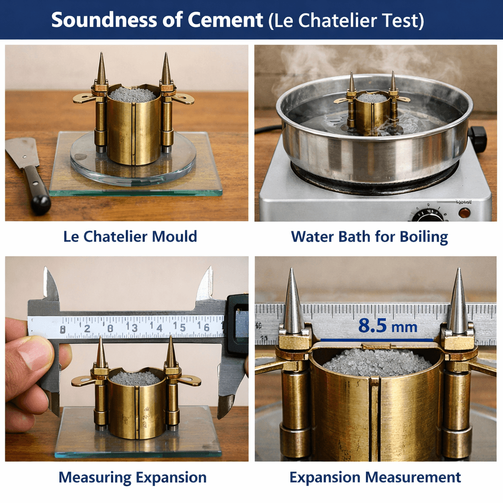
Soundness Test of Cement – Le Chatelier Method Author: Kishor Kumar · Updated: February 2026 · Read time: ~8 minutes 1. Introduction The Soundness Test of Cement ensures that cement does not undergo excessive expansion after setting, which can cause cracks in concrete and structural failure. The Le Chatelier Method specifically measures expansion due to free lime (CaO) or magnesia content. 2. Purpose Check dimensional stability of cement Detect presence of free lime (CaO) or magnesia Prevent cracking in concrete structures Ensure compliance with IS 4031 Part 3 and MoRTH specifications 3. Applicable Standards IS 4031 (Part 3) – Soundness test of cement using Le Chatelier method IS 4031 (Part 4) – Standard consistency for paste MoRTH Specifications – Cement quality control 4. Apparatus Le Chatelier Mould (split ring, inner & outer arcs) Vernier Caliper – for measuring expansion Water Bath / Beaker – 27–30°C Glass Plate / Base Plate Mortar Preparation Tools (trowel, spatula) 5. Test Sample Preparation Cement paste is prepared using standard consistency water. Example ratio: 1 part cement : 0.78 parts water (by weight). Sample Preparation Example: For 100 g of cement: Water required = 100 × 0.78 = 78 g Mix cement and water to obtain a uniform paste for filling the Le Chatelier mould. 6. Test Procedure – Le Chatelier Method Preparation of Cement Paste Determine the standard consistency of cement using IS 4031 (Part 4). Mix cement and water (~1:0.78 by weight) to obtain uniform paste. Avoid lumps to ensure accurate test results. Filling the Le Chatelier Mould Clean mould thoroughly and lightly oil to prevent sticking. Fill mould carefully, avoiding air pockets. Tap gently or use spatula to compact paste evenly. Leveling the Paste Level top of paste to match upper rim of mould. Ensure flush surface to avoid erroneous readings. Immersion in Water Bath Place mould in water bath maintained at 27–30°C for 24 hours. Keep undisturbed and maintain constant temperature. Measurement of Expansion Remove mould carefully after 24 hours. Measure distance between indicator arms using vernier caliper. Take measurements to nearest 0.5 mm for precision. Calculation of Expansion Formula: Expansion (mm) = Final distance between arms – Original distance between arms Record mean of two measurements if multiple moulds are tested for accuracy. 7. Acceptance Criteria Maximum expansion for OPC: ≤ 0.8 mm (IS 4031 Part 3) Rapid Hardening Cement: slightly lower limits 8. Engineering Significance Prevents cracks in concrete due to excessive expansion Ensures dimensional stability of cement in structural and pavement applications Critical for highway pavements, bridges, and high-rise concrete structures 9. Common Mistakes Air bubbles while filling mould Incorrect water bath temperature Improper vernier caliper measurement Using non-standard consistency paste Ensure proper handling to avoid false readings; repeat test if inconsistent. 10. Frequently Asked Questions What is the purpose of the Le Chatelier test? It checks cement expansion due to free lime or magnesia, ensuring dimensional stability. Which IS code covers the test? IS 4031 (Part 3) What is the maximum allowable expansion? ≤ 0.8 mm for Ordinary Portland Cement (OPC) How is cement paste prepared? Using standard consistency water; example ratio: 1 part cement : 0.78 parts water by weight. What happens if expansion exceeds the limit? Excessive expansion indicates free lime; cement should be rejected or used with caution in structural work. 11. Conclusion The Soundness Test of Cement – Le Chatelier Method ensures cement stability, prevents cracks, and guarantees compliance with IS 4031 and MoRTH specifications. Always perform this test for critical concrete and pavement works. Written by: Kishor Kumar · Civil / Highway Engineer – QA/QC & Site Execution · Source: HighwayQualityTest.com 🧪 Complete Cement Laboratory Test Series IS 4031 IS 516 MoRTH NHAI QA/QC These laboratory tests are conducted sequentially for complete cement and concrete quality verification in highway, bridge, structure, and rigid pavement works as per IS 4031, IS 516, MoRTH Specifications, and NHAI Quality Assurance Protocols. 🔬 Fineness of Cement IS 4031 (Part 1) Sieve analysis and Blaine air permeability method for determining cement particle fineness. ⚙️ Standard Consistency IS 4031 (Part 4) Determination of optimum water percentage using Vicat apparatus. ⏱️ Initial Setting Time IS 4031 (Part 5) Measures the beginning of cement hardening using Vicat needle penetration. 🧱 Final Setting Time IS 4031 (Part 5) Determines the complete hardening stage of cement paste. 💪 Compressive Strength IS 4031 (Part 6) Mortar cube crushing strength evaluation at different curing ages. 🏗️ Concrete Cube Test IS 516 Concrete compressive strength testing for site quality control and mix validation. 📌 Quality Control Insight These tests must be conducted in proper sequence to establish correlation between cement fineness, water demand, setting characteristics, and strength development during highway, bridge, and structural concrete works—especially under NHAI, MoRTH, and independent third-party QA/QC audits. HIGHWAY QUALITY TEST Download Soundness of Cement Test Excel Format Prepare professional Soundness of Cement test reports in minutes using our ready-to-use Excel format with automatic calculations. Accurately determine the soundness of cement using the Le Chatelier Method and generate laboratory-ready reports while eliminating manual calculation errors. 💰 Only ₹99 One-Time Payment • Instant Access • Lifetime Access 🛒 Buy Soundness of Cement Excel Format ✔ Secure Payment   |   ✔ Instant Download   |   ✔ Editable Excel

Soundness Test of Cement – Le Chatelier Method Read More »

Cement
Los Angeles Abrasion Test Apparatus

Los Angeles Abrasion Test IS 2386 Part IV

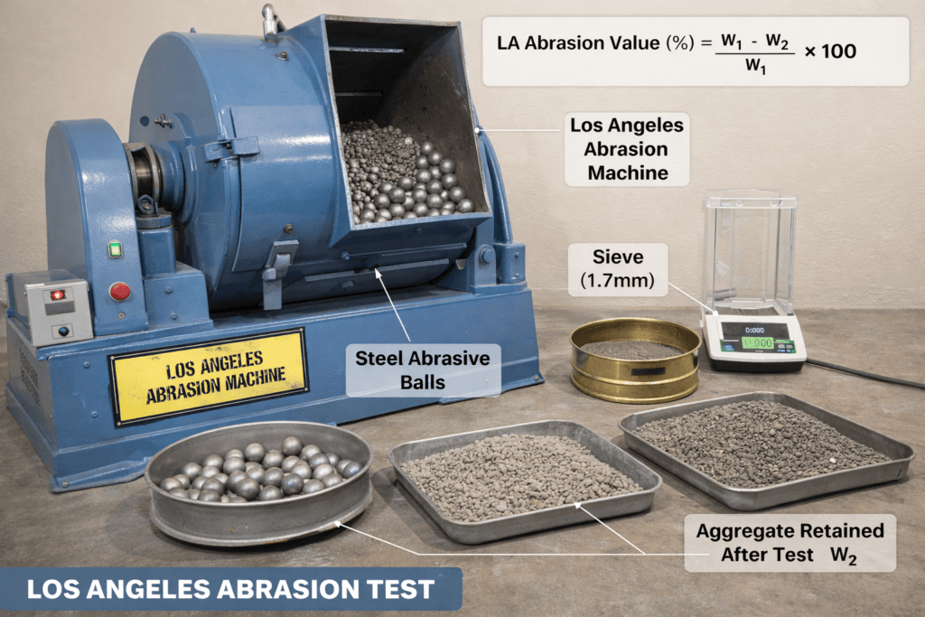
Los Angeles Abrasion Test – Procedure, Calculation, Apparatus & Limits (IS 2386 Part IV) The Los Angeles Abrasion Test is one of the most important tests used to evaluate the toughness and abrasion resistance of coarse aggregates used in road construction and concrete works. This test determines how aggregates behave when subjected to wear, impact and grinding action. Aggregates with high abrasion resistance ensure longer pavement life, better durability and reduced maintenance costs. The test is conducted according to IS 2386 (Part IV) – Methods of Test for Aggregates and is also specified in MoRTH Specifications for Road and Bridge Works (5th Revision, 2013). Importance of Los Angeles Abrasion Test in Highway Engineering Aggregates are the primary load-bearing material in flexible pavements. When traffic loads move over pavement surfaces, aggregates are continuously subjected to: Abrasion due to tyre friction Impact from moving vehicles Grinding action between aggregate particles If aggregates are weak, they will break into smaller particles, causing: Pavement rutting Loss of surface texture Premature road failure The Los Angeles Abrasion Test helps engineers select durable aggregates suitable for highway construction. Objective of the Test The main objectives of the Los Angeles Abrasion Test are: To determine the abrasion resistance of aggregates To measure the toughness of aggregates To evaluate the quality of aggregates for road works To ensure aggregates meet MoRTH specifications Relevant Standards IS 2386 (Part IV) – 1963 Methods of test for aggregates for concrete. MoRTH Specifications (2013) Specifications for road and bridge works. ASTM C131 / ASTM C535 International standards for abrasion testing. Apparatus Required for Los Angeles Abrasion Test Los Angeles Abrasion Machine Hollow steel drum Internal diameter: 700 mm Length: 500 mm Rotational speed: 30–33 rpm Steel Abrasive Balls Diameter: 48 ± 2 mm Weight: 390 – 445 g each Hardness: 400 – 450 HB IS Standard Sieves Weighing Balance (accuracy 1 g) Drying Oven (105 – 110°C) Tray and sieve brush Sample Preparation Proper sample preparation is essential for accurate test results. The following steps should be followed: Collect representative aggregate samples. Wash aggregates to remove dust and impurities. Dry the aggregates in an oven at 105–110°C. Allow the sample to cool to room temperature. Weigh the required sample weight (usually 5000 g). Grading of Aggregates for the Test Grading Aggregate Size (mm) Sample Weight (g) No. of Revolutions Typical Use A 63 – 50 5000 500 Granular Sub Base B 50 – 40 5000 500 WMM Base C 40 – 25 5000 500 Dense Bituminous Macadam D 25 – 20 5000 500 Bituminous Macadam E 20 – 12.5 5000 1000 Bituminous Concrete Test Procedure PROCEDURE – LOS ANGELES ABRASION TEST Clean aggregates dried in an oven at 105–110°C shall be used for testing. The grading used in the test should be nearest to the grading to be used in the construction. Aggregates weighing 5 kg for grading A, B, C or D and 10 kg for grading E, F or G may be taken as test specimen and placed in the cylinder. Choose the abrasion charge depending on the grading of the aggregate and place in the cylinder of the machine. Fix the cover dust tight and rotate the machine at a speed of 30 to 33 revolutions per minute. The machine shall be rotated for 500 revolutions for grading A, B, C and D, and for grading E, F and G it shall be rotated for 1000 revolutions. After the desired number of revolutions, stop the machine and discharge the material from the machine taking care to take out entire stone dust. Using a sieve of size 1.70 mm IS Sieve, the material is first separated into two parts and the finer portion is taken out and sieved further on a 1.70 mm IS Sieve. The portion of material coarser than 1.70 mm size is washed and dried in an oven at 105–110°C to constant weight and weighed correct to one gram. Calculation of Los Angeles Abrasion Value The Los Angeles abrasion value is calculated using the following formula: Los Angeles Abrasion Value (%) = ((A − B) / A) × 100 Where: A = Original weight of sample (g) B = Weight retained on 1.70 mm sieve after test (g) Example Calculation Initial weight of sample = 5000 g Weight retained after test = 3600 g Abrasion Value = ((5000 − 3600) / 5000) × 100 Abrasion Value = 28% Permissible Limits as per MoRTH Layer Maximum LA Abrasion Value Granular Sub Base 45% Base Course 40% Bituminous Layers 35% Wearing Course 30% Advantages of the Test Simple and widely used method Provides reliable measure of aggregate toughness Essential for pavement design Helps maintain highway quality control Limitations of the Test Does not fully simulate field traffic conditions Results may vary for soft aggregates Not suitable for very small aggregates Frequently Asked Questions (FAQ) What is the Los Angeles Abrasion Test? It is a laboratory test used to determine the resistance of aggregates to abrasion and impact. What is the maximum permissible abrasion value? For wearing courses in highways, the maximum value is typically 30%. Which IS code specifies the test? The test is specified in IS 2386 (Part IV). What does a lower abrasion value indicate? Lower abrasion value means stronger and more durable aggregates. Related Aggregate Tests for Highway & Concrete Works Explore detailed test procedures, calculations and acceptance criteria as per IS, MoRTH & IRC specifications: ✅ Aggregate Impact Value (AIV) Test – Toughness of Aggregates ✅ Los Angeles Abrasion Test – Wear & Abrasion Resistance ✅ Aggregate Crushing Value (ACV) Test – Strength Evaluation ✅ Flakiness & Elongation Index Test – Shape Characteristics ✅ Water Absorption Test – Durability & Porosity Check 📌 Pro Tip: Use AIV, ACV, Los Angeles Abrasion, and Shape & Water Absorption Tests together to ensure aggregate suitability for bituminous layers & cement concrete as per MoRTH Section 400 & 500. HIGHWAY QUALITY TEST Download Los Angeles Abrasion Test Excel Format Prepare professional Los Angeles Abrasion (LAA) test reports in

Los Angeles Abrasion Test IS 2386 Part IV Read More »

Aggregate
aggregate crushing value test

Aggregate Crushing Value Test

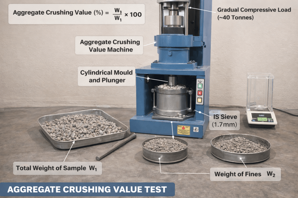
Aggregate Crushing Value Test — Procedure, Calculation & Limits | QC for Pavements Aggregate Crushing Value (ACV) Test — Procedure, Calculation & Acceptance Limits Quick lab method for QC of aggregates used in concrete pavements — Field & Lab Overview The Aggregate Crushing Value (ACV) test measures the resistance of an aggregate sample to crushing under a gradually applied compressive load. The result helps determine suitability of aggregates for different pavement layers and wearing surfaces. Why This Test Matters in Highway Construction In highway and pavement engineering, aggregates form the backbone of structural layers such as Sub-Base, Base, and Surface Courses. Their strength directly influences the ability of pavements to resist traffic loads, impacts, and repeated loading without excessive crushing or breakdown. The Aggregate Crushing Value (ACV) test provides a relative measure of the resistance of aggregates to crushing under gradually applied compressive loads, as defined by IS 2386 (Part IV). Aggregates with a low ACV (i.e., lower percentage of fines) indicate higher strength and durability, which is critical for long-lasting road surfaces and reduced maintenance costs. As per standard practice, the ACV of aggregates used in wearing surfaces (e.g., concrete pavements) should be controlled rigorously to ensure structural performance over the design life. Aggregates failing this test may lead to premature rutting, surface degradation, and loss of serviceability. Apparatus Item Specification / Notes Steel cylindrical measure Internal diameter 115 mm, height 180 mm Plunger / piston Diameter 150 mm (for main apparatus) Tamping rod Diameter 16 mm (rounded end), length 450–600 mm Balance Capacity ≈ 3 kg with 0.01 g accuracy Compressive testing machine 40 tonnes capacity, uniform loading rate 4 tonnes/min IS sieves 12.5 mm, 10 mm, and 2.36 mm Sample Selection & Preparation Use aggregate passing 12.5 mm and retained on 10 mm IS sieve. Ensure the aggregates are surface-dry (no visible free moisture). Sample weight: as required by the cylinder capacity — record dry weight (W1). Procedure (Step-by-step) The aggregate passing 12.5 mm IS sieve and retained on 10 mm IS sieve shall be selected for standard test. The aggregate should be in surface dry condition before testing. The cylindrical measure shall be filled by the test sample of aggregate in three layers of approximately equal depth, each layer being tamped 25 times by the rounded end of the tamping rod. After the third layer is tamped, using the tamping rod as a straight edge levels off the aggregate at the top of the cylindrical measure. Weigh the sample and repeat the test for another trial. The cylinder of the test apparatus shall be placed in position on the base plate; place one third of the test sample in this cylinder and tamp 25 times by the tamping rod. Similarly, the other two parts of the test specimen are added, each layer being subjected to 25 blows. The surface of the aggregates shall be levelled and insert the plunger so that it rests on this surface in level position. Keep the cylinder with the test sample and the plunger in position and place on the compression testing machine. Load is then applied through the plunger at a uniform rate of 4 tons per minute until the total load is 40 tonnes, and then release the total load. Remove the aggregates including the crushed portion from the cylinder and sieve on a 2.36 mm IS sieve. Collect the material, which passes this sieve. The above crushing test shall be repeated on second sample of the same weight in accordance with above test procedure. Thus two tests are made for the same specimen for taking an average value. Calculation Aggregate Crushing Value (ACV) is the percentage ratio of crushed fines to the total sample weight. Aggregate Crushing Value = (W2 / W1) × 100 Where: W1 = Total dry weight of sample W2 = Weight of material passing 2.36 mm IS sieve Report: Mean of two test results Results & Reporting Report the mean of the two test values as the final ACV for the aggregate sample. Include: Sample identification and date Apparatus used and calibration status W1 and W2 values for both trials and the mean ACV Any deviations from standard procedure Acceptance Limits Application Maximum ACV (%) Cement concrete pavements 30 Wearing surfaces 45 Frequently Asked Questions Why do we use a 2.36 mm sieve for fines? 2.36 mm is the standard IS limit for defining crushed fines in this test — it provides a consistent basis to compare strength characteristics across aggregate sources. What if my aggregate grading differs? If grading is outside the specified range (12.5–10 mm) use a representative fraction or follow the standard practice for coarse/fine fractions as specified in the relevant code. Notes & Best Practices Always run two trials and report the mean to reduce random error. Ensure the compression machine platen and the plunger are clean and parallel before applying load. Record ambient conditions and any visible degradation of sample during handling. Quick Checklist Aggregate: 12.5–10 mm Tamping: 25 blows/layer Loading: 4 t/min to 40 t Sieve for fines: 2.36 mm Acceptable ACV: <=30% (concrete pavements) Useful snippets <strong>ACV = (W2 / W1) × 100</strong> Use this procedure HIGHWAY QUALITY TEST Download Aggregate Crushing Value (ACV) Test Excel Format Prepare professional Aggregate Crushing Value (ACV) test reports in minutes using our ready-to-use Excel format with automatic calculations. Eliminate manual calculation errors and generate laboratory-ready reports instantly. 💰 Only ₹99 One-Time Payment • Instant Download • Lifetime Access 🛒 Buy ACV Test Excel Format ✔ Secure Payment   |   ✔ Instant Download   |   ✔ Editable Excel 🚀 BEST VALUE Upgrade to the Complete Aggregate Testing Excel Toolkit Need more than one Excel format? Save money with our Complete Aggregate Testing Excel Toolkit containing 19 professional Excel formats with automatic calculations, laboratory-ready observation sheets and printable reports. Why Buy the Complete Toolkit? ✔ One Excel Format = ₹99 ✔ 6 Individual Formats = ₹594 ✔ 10 Individual Formats = ₹990 ✔ 19 Individual Formats = ₹1,881 Get

Aggregate Crushing Value Test Read More »

Aggregate

Free Swell Index (FSI) Test – Procedure, Formula & Acceptance Criteria (IS 2720 Part 40)

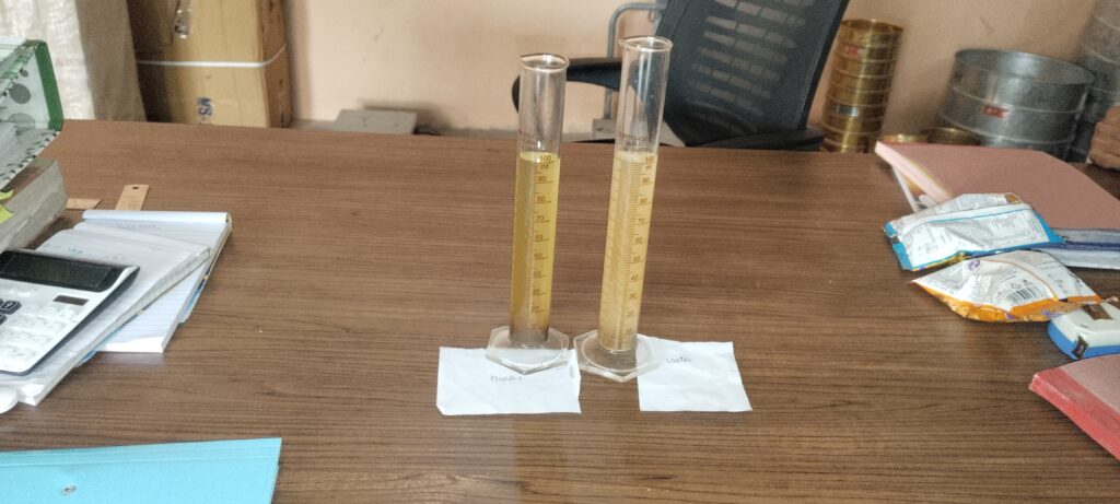
Explore all Soil Tests: Soil Testing Hub Home » Geotechnical Tests » Free Swell Index (FSI) Test Free Swell Index (FSI) Test – Procedure, Formula & Acceptance Criteria (IS 2720 Part 40) Test Standard: IS:2720 (Part 40) | Applicable Codes: MoRTH, IRC:75 (2015), IRC:SP:89 What is Free Swell Index (FSI) Test? The Free Swell Index (FSI) test is a laboratory test used to determine the swelling potential of soil when immersed in water under unconstrained conditions. It helps in identifying expansive soils containing clay minerals such as montmorillonite. Why it matters: High Free Swell Index values may lead to pavement heaving, cracking, and loss of subgrade stability if the soil is used without treatment. Scope & Applicable Standards IS:2720 (Part 40) – Determination of Free Swell Index of Soil MoRTH Section 300 – Subgrade and Earthwork IRC:75 (2015) – Guidelines for Embankments and Subgrades IRC:SP:89 – Soil Testing in Road Works NHAI QA/QC Manual Apparatus Required for FSI Test 425 micron IS sieve Two 100 ml graduated glass cylinders (IS:878) Oven maintained at 110 ± 5 °C Electronic balance with 0.01 g accuracy Distilled water and kerosene Glass rod, spatula and weighing dishes Free Swell Index Test Procedure (IS 2720 Part 40) Take about 500 g of air-dried soil and sieve it through a 425-micron sieve. Weigh two soil samples of 10 g each. Place one sample in each 100 ml graduated cylinder. Fill one cylinder with kerosene and the other with distilled water up to the 100 ml mark. Stir gently to remove entrapped air bubbles. Allow the samples to stand undisturbed for 24 hours at 27 ± 2 °C. Record the final soil volumes: Vk = Volume of soil in kerosene Vw = Volume of soil in water Free Swell Index Formula FSI (%) = [(Vw – Vk) / Vk] × 100 FSI Interpretation and Acceptance Criteria Free Swell Index (%) Swelling Nature Suitability for Subgrade 0 – 20 Low Suitable for direct use 20 – 50 Moderate Use with control measures Above 50 High to Very High Stabilization or replacement required Note: Free Swell Index is an index test and should be used along with Atterberg limits and swell pressure tests for design decisions. Precautions During FSI Test Ensure glass cylinders are clean and dry. Maintain the specified test temperature. Do not disturb the samples during the standing period. Record volume readings accurately. Frequently Asked Questions Is Free Swell Index the same as swell pressure? No. Free Swell Index measures volume increase without restraint, whereas swell pressure measures pressure developed under confinement. Can Free Swell Index alone be used for soil design? No. It is only an indicator test and must be supported by other geotechnical tests. How can expansive soil be treated? Common methods include lime stabilization, cement stabilization, blending with non-expansive soil, or soil replacement. References: IS:2720 (Part 40), MoRTH Specifications, IRC:75 (2015), IRC:SP:89 © 2025 Highway Quality Test HIGHWAY QUALITY TEST Download Free Swell Index Test Excel Format Prepare professional Free Swell Index Test reports in minutes using our ready-to-use Excel format with automatic calculations. Accurately determine the Free Swell Index (FSI) of expansive soils while eliminating manual calculation errors and generating laboratory-ready reports instantly. 💰 Only ₹99 One-Time Payment • Instant Access • Lifetime Access 🛒 Buy Free Swell Index Excel Format ✔ Secure Payment   |   ✔ Instant Download   |   ✔ Editable Excel

Free Swell Index (FSI) Test – Procedure, Formula & Acceptance Criteria (IS 2720 Part 40) Read More »

Soil

Water Absorption Test

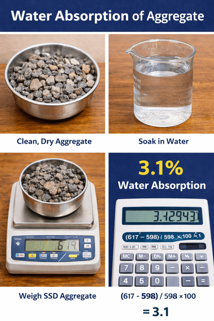
Water Absorption Test of Coarse Aggregate — Objective, Procedure & Calculation Water Absorption Test of Coarse Aggregate The Water Absorption Test determines the percentage of water absorbed by coarse aggregates, providing an indication of pore structure, density, and suitability for high-quality concrete and asphalt works. Objective To determine the Water Absorption (%) of a coarse aggregate sample using SSD and Oven-dry mass values. Apparatus Required Tray or suitable container Balance (Capacity ≥ 3 kg, Accuracy 0.5 g) Oven (100–110°C) Cotton cloth Test Procedure 1. Immersion (Saturation) Take at least 2000 g (2 kg) of aggregate. Immerse in clean water for 24 hours to fill internal pores. 2. Saturated Surface Dry (SSD) Condition Remove the sample and wipe gently with a cotton cloth. Ensure no visible free water film remains on the surface. Weigh the sample → SSD Mass (A). 3. Oven Drying Place SSD sample in oven at 100–110°C for 24 hours. Cool it and weigh → Oven‑Dry Mass (B). 4. Repeat Trial Repeat the procedure on another sample and take the average. Calculation Water Absorption (%) = (A − B) / B × 100 Where: A = SSD Mass of aggregate B = Oven‑Dry Mass of aggregate Example If: A (SSD Mass) = 2045 g B (Oven-Dry Mass) = 2000 g Water Absorption (%) = (2045 − 2000) / 2000 × 100 = 45 / 2000 × 100 = 2.25% Importance in Construction Mix Design Adjustments: Highly absorptive aggregates steal mix water → affects workability. Durability: Higher absorption = higher porosity → weaker freeze-thaw and weathering resistance. ✔️ Typical Acceptable Limits Aggregate Type Max Water Absorption (%) Coarse Aggregate (Normal concrete) ≤ 2% Fine Aggregate (Sand) ≤ 3% For high-performance or severe exposure concrete, stricter limits may apply. Background & Standard Reference The Water Absorption Test is covered under IS 2386 (Part 3) – Specific Gravity, Density, Voids, Absorption and Bulking. This test provides insight into the internal pore structure of aggregates, which directly affects concrete durability, water demand, and long‑term performance. Aggregates with excessive pores tend to absorb more water, which may lead to reduced compressive strength and increased shrinkage. By determining absorption, engineers calibrate mix water content accurately to achieve the target workability and strength parameters. Factors Affecting Water Absorption Aggregate Type: Crushed rock typically has lower absorption than natural aggregates. Surface Texture: Rough, angular particles may retain more surface moisture. Pore Structure: Aggregates with interconnected pores have higher absorption levels. Weathering: Older, weathered aggregates tend to be more porous. Mineral Composition: Some minerals inherently exhibit higher porosity. Significance of SSD Condition The SSD (Saturated Surface Dry) condition is critical because it represents the state where internal pores are full of water while the exterior surface is dry. This allows mix water calculations to remain accurate. If aggregates are not brought to SSD before batching, they either absorb mix water (leading to lower workability) or contribute excess water (making the mix too wet). The SSD condition ensures correct water‑cement ratio, the single most important factor governing concrete strength. Impact on Concrete Performance Water absorption is directly linked to aggregate quality. Aggregates with low absorption are denser and more durable, making them suitable for high‑strength and long‑life structures. On the other hand, aggregates with high absorption may lead to increased permeability, reduced freeze‑thaw resistance, and potential durability issues. Additionally, when absorption is high, the concrete mix becomes unpredictable without proper adjustments, affecting slump, cohesiveness, and compaction. Precautions Ensure aggregates are completely submerged during the 24‑hour soaking period. Wipe surface moisture gently—over‑drying may lead to inaccurate SSD readings. Do not exceed oven temperature beyond 110°C to avoid thermal damage. Use a calibrated balance for precise mass measurements. Allow oven‑dry samples to cool in a desiccator if available, to prevent moisture uptake from air. Notes for Field Engineers In site conditions, aggregates stored in open yards exhibit varying levels of moisture. Regular absorption testing helps determine free moisture correction during batching to maintain consistent mix quality. For automated batching plants, entering accurate absorption values ensures the batching software adjusts water content correctly. This prevents issues such as plastic shrinkage, excessive bleeding, or segregation in fresh concrete. IS Code References IS Code Description IS 2386 (Part 3) Methods of Test for Aggregates – Specific Gravity, Density, Voids & Water Absorption IS 383 Specification for Coarse and Fine Aggregates for Concrete IS 456 General concrete requirements & material quality guidance Frequently Asked Questions (FAQ) 1. What is a good water absorption value for coarse aggregates? For most concrete works, water absorption should be ≤ 2%. Lower values indicate denser and more durable aggregates. 2. Why is SSD condition important? SSD ensures that aggregate pores are filled without free surface water. This prevents errors in mix design water calculations. 3. Can high water absorption affect concrete strength? Yes. Aggregates with high absorption draw water from the concrete mix, reducing effective W/C ratio and causing poor workability and potential strength loss. 4. How often should this test be performed? Typically during material approval and periodically during construction to ensure consistent aggregate quality. 5. Do different rocks have different absorption characteristics? Yes. Dense rocks like basalt and granite have low absorption. Porous rocks like sandstone and lightweight aggregates have higher absorption. HIGHWAY QUALITY TEST Download Water Absorption Test Excel Format Prepare professional Water Absorption Test reports with automatic calculations for Coarse Aggregates (40 mm, 20 mm, 10 mm), Sand, and Stone Dust. Save time, eliminate manual errors, and generate laboratory-ready reports instantly. ✅ What’s Included Automatic Water Absorption Calculations 40 mm Aggregate Format 20 mm Aggregate Format 10 mm Aggregate Format Sand Water Absorption Format Professional Laboratory Report Layout Print Ready (A4 Size) Editable Excel (.xlsx) Instant Download Lifetime Access 👷 Perfect For Highway Engineers Civil Engineers QA/QC Engineers Material Testing Laboratories Consultants Engineering Students 💰 Bundle: ₹149 Only CA (40,20,10 mm + Sand) + Stone Dust • One-Time Payment • Instant Access 🛒 Buy CA (40,20,10 mm + Sand) Excel – ₹99 🛒 Buy Stone Dust Excel – ₹49 ✔ Secure Payment  

Water Absorption Test Read More »

Aggregate

© 2026 HIGHWAY QUALITY TEST. All rights reserved.

WhatsAppNeed Help?
Scroll to Top